Basic Statistics for reliability and mortality concepts

therefore the survival function tells us the probability that a component can still be operational and functioning after a generic time t. There are different types of survival curves (discrete, continuous or mixed). In general a survival function must have the following characteristics:

For simplicity in the following, we will only deal with the cases of continuous and differentiable functions.

we can express this probability by subtracting from the probability that the lifespan of the component is less than or equal to t+dt the probability that the lifespan is less than or equal to t: but the two terms on the right-hand side of the equation are two terms of the statistical mortality function ϕ. therefore the probability density of the duration of a component is the derivative of mortality over time ϕ

Now to continue with the mathematical treatment and obtain the failure rate function, let’s consider the case in which the probability law that governs the failure of the component under observation is discrete and not continuous. For example, this is the case when on the x-axis of time there are days or weeks that do not have a continuous trend. The time variable t therefore takes on the values N={0,1,2,3,4….}. The probability that a component will fail on date n+1 + is given by the formula:

P(T=n+1)= P(T\leq n+1) - P(T\leq n)

therefore meaning that the probability that the component fails exactly on date n+1 is given by the difference between the cumulative probability that the component fails by that date minus the cumulative probability that it fails on the immediately preceding date. But we previously called this cumulative probability as the statistical mortality of the component (ϕ function). We can therefore write:

P(T=n+1)= P(T\leq n+1) - P(T\leq n) = \phi(n+1) - \phi (n)

Similarly we can write the same probability in terms of the survival function:

P(T=n+1)= P(T\leq n+1) - P(T\leq n) = (1-P(t>n+1))- (1-P(t>n)) =P(t>n)-P(t>n-1) =\\\,\\= v(n) - v(n+1)

Let us return to the case in which the probability of component failure is continuous as a function of time. We can write:

P(t< T\leq t+dt) = P(T >t) P(T \leq t+dt |T>t)

that is, the probability that the failure occurs in the time interval )t, t+dt( is given by the product of the probability that this occurs beyond t and the probability that it occurs before t+dt under the condition (we have a conditional probability!) that did not happen before t. Let’s isolate the conditional probability:

P(T \leq t+dt |T>t) = \frac{P(t< T\leq t+dt)}{P(T >t) } = \frac{i}

the amount:

it is called the instantaneous failure rate and expresses the probability that a component fails in the interval )t,t+dt( knowing (therefore under the condition) that the component was in good condition at time t. The product of the lambda function for an interval of time it provides us with the ratio between the number of components that fail in that interval and the good ones at the beginning of the interval itself. This function has the characteristic of not being able to take on negative values (which would mean that healthy components over time) and can be non-monotonic and in any case can be increasing or decreasing.

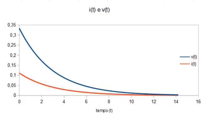
which means that if the lambda function is constant over time, the survival law is a simple exponential law. If, however, the lambda function is linearly increasing, then the survival curve is a bell curve truncated at time t=0.

The integral present at the exponent of the exponential represents the cumulative function of the failure rate

Expected value and variance of the law of survival

To calculate the expected value and variance of the survival law, simply apply the generic formulas of these moments of the function. Remember that a generic moment is given by: